Article Text

Abstract
Objective We aim to explain the unadjusted, adjusted and marginal number needed to treat (NNT) and provide software for clinicians to compute them.
Methods The NNT is an efficacy index that is commonly used in randomised clinical trials. The NNT is the average number of patients needed to treat to obtain one successful outcome (ie, response) due to treatment. We developed the nntcalc R package for desktop use and extended it to a user-friendly web application. We provided users with a user-friendly step-by-step guide. The application calculates the NNT for various models with and without explanatory variables. The implemented models for the adjusted NNT are linear regression and analysis of variance (ANOVA), logistic regression, Kaplan-Meier and Cox regression. If no explanatory variables are available, one can compute the unadjusted Laupacis et al’s NNT, Kraemer and Kupfer’s NNT and the Furukawa and Leucht’s NNT. All NNT estimators are computed with their associated appropriate 95% confidence intervals. All calculations are in R and are replicable.
Results The application provides the user with an easy-to-use web application to compute the NNT in different settings and models. We illustrate the use of the application from examples in schizophrenia research based on the Positive and Negative Syndrome Scale. The application is available from https://nntcalc.iem.technion.ac.il. The output is given in a journal compatible text format, which users can copy and paste or download in a comma-separated values format.
Conclusion This application will help researchers and clinicians assess the efficacy of treatment and consequently improve the quality and accuracy of decisions.
- schizophrenia & psychotic disorders
Statistics from Altmetric.com
Introduction
The number needed to treat (NNT) refers to the average number of patients needed to treat to obtain one response due to treatment.1 The NNT is a widely used efficacy index in randomised clinical trials.2 In computing the NNT, it is assumed that the outcome is dichotomous and may be successful or unsuccessful (reflecting treatment responders or non-responders, respectively). We start by introducing the unadjusted, adjusted and marginal NNT. We illustrate their use in selected scenarios and present a software application to compute the NNT for clinicians.
Scenario 1: illustration of the unadjusted NNT
The unadjusted NNT is suitable for settings without explanatory variables since it is calculated only with the outcome variable. The probability of response due to treatment is defined as the probability of a successful outcome minus the probability of a successful outcome due to a placebo response. Assume, for example, that the probability of response due to treatment is 1. Namely, it is sufficient to treat one patient to observe a response due to treatment, thus NNT=1. Consider now that the probability of response due to treatment in the target population is 0.5. In this case, on average, two patients are needed to be treated to observe one response due to treatment. As such, the NNT is defined as 1/0.5=2. In other words, the lower the treatment efficiency, the larger the NNT. The best possible NNT is 1, which corresponds to perfect treatment efficacy. Analogically, the worst possible NNT is infinity, which corresponds to an ineffective treatment that is indistinguishable from a placebo effect. The response variable can be defined as a relative reduction of the endpoint Positive and Negative Syndrome Scale (PANSS) Score3 compared with the baseline PANSS Score. The PANSS total score is based on positive, negative and general psychopathological symptoms of schizophrenia. The PANSS consists of 30 items, each rated on a scale of 1 to 7. Therefore, the overall score that comprises the PANSS Index takes integer values between 30 and 210.
There are three available estimators of the unadjusted NNT. The first estimator is Laupacis et al’s non-parametric estimator, while this is a robust estimator, it does not use all the available information in the sample.1 The second NNT is Furukawa and Leucht’s estimator, which is appropriate to use only for normally distributed outcomes with equal standard deviations (SD).4 The third estimator is the parametric estimator proposed by Vancak et al.5 When the parametric model is correctly specified, this estimator is the optimal NNT because it adapts to the outcome variable distribution and uses all the available information in the sample.
Scenario 2: illustration of the adjusted and marginal NNT
To extend the unadjusted NNT, the adjusted and the marginal NNT account for explanatory variables. Assume, for example, that in addition to the outcome variable, we are willing to adjust the NNT to an explanatory variable, such as the baseline PANSS Score. Assume that the probability of response due to treatment depends on the PANSS baseline score6; hence, it requires adjustment. Assume, for example, that for clinical reasons we discriminate between two subpopulations: group A with a PANSS baseline score of >80, which corresponds to moderately ill and higher symptom severity levels, and group B with a PANSS baseline score of <80, which corresponds to a normal up to mildly ill symptom severity levels.7 Assume that the probability of response due to treatment for group A is 0.75 and for group B is 0.25. Therefore, the adjusted NNTs are 1.25, and 4, respectively (ie, 1/0.75=1.25 and 1/0.25=4).
The marginal NNT is defined as the NNT based on the marginal probability of success due to treatment. The marginal probability of success due to treatment is the probability that marginalises out the covariates. Namely, by taking the weighted average of the response probabilities over all possible adjustments, we obtain the marginal probability of success. According to our example, assume that the study population consists of 50% of group A and 50% of group B. In such a case, the weighted average probability of success due to treatment is the average of the given probabilities, which is 0.5. Therefore, the marginal NNT is 1/0.5=2. Consider, for instance, the marginal NNT with a different distribution of the target population where only 20% of the population are of group A, while 80% are of group B. Namely, there is a probability of 0.2 that a randomly drawn participant from this population is of group A and of 0.8 that he is of group B. Therefore, the marginal probability of success due to treatment is the weighted average of the probabilities mentioned above (ie, 0.75, and 0.25 for groups A and B, respectively)

Hence, the marginal NNT is 1/0.35 ≈ 2.86. Notably, the marginal NNT is not the weighted average of the adjusted NNTs, but the reciprocal of the weighted average of the adjusted probabilities of response due to treatment. This distinction plays a key role, as averaging the NNTs may result in wrong calculations and conclusions. In summary, where we account for the distribution of the explanatory variables in the calculation of the NNT, we obtain the marginal NNT. Additionally, where we adjust the NNT for a particular value of the explanatory variables, the calculated NNT is the adjusted NNT.
Scenario 3: illustration of the NNT in survival analysis
In survival analysis, the outcome variable is the time from the beginning of follow-up to the event. The event may be the time until death, the time to recover or any other event of interest. For each timepoint, the successful outcome is defined as remaining in the trial at least to this timepoint. For example, assume that we have a treatment course for schizophrenia with two follow-up visits (eg, 9 and 15 months after baseline). The outcome variable is time to discontinuation of the treatment for any reason. In the Clinical Antipsychotic Trials of Intervention Effectiveness8 schizophrenia trial, most patients discontinued their treatment due to inefficacy or intolerable side effects.9 Assume that 50% of the initial sample survived due to treatment up to the first follow-up visit and 25% up to the second visit. Namely, there is a probability of 0.5 to survive due to treatment up to the first visit and 0.25 up to the second visit. Therefore, the NNT at the time of the first visit is 1/0.5=2, and so at the time of the second visit, the NNT is 1/0.25=4. Next, assume that, as in the previous example, we have two groups A and B, which corresponds to the same baseline PANSS Score as in scenario 2. In addition, assume that group A responds much better to the treatment than group B. For example, assume that there is the same number of participants in both groups. Hence, there is a probability of 0.5 that randomly drawn participants from this sample are of group A or group B. However, the survival rate of group A at the time of the first visit is 75% (ie, probability of 0.75), while the survival rate of group B at the same time is only 25% (ie, probability of 0.25). Thus, the adjusted NNTs at the time of the first visit are 1/0.75=1.25 and 1/0.25=4 for groups A and B, respectively. While the marginal survival rate at this timepoint is the weighted average of the probabilities

Hence, the marginal NNT at the time of the first visit is 1/0.5=2. Assume, for the second visit, that the survival rate for group A is 0.4, while for group B is 0.1. Therefore, the adjusted NNTs for groups A and B are 1/0.4=2.5 and 1/0.1=10, respectively. The marginal survival rate at the second visit is 0.25 (ie,  ), thus the marginal NNT is 1/0.25=4. Another aspect that characterises survival data is censoring (ie, premature dropout). Namely, we may not observe the event (treatment discontinuation) due to loss of follow-up or for other reasons. In other words, we assume that all clinical trial study participants start simultaneously, but some are censored before the end of the trial (ie, prematurely dropout). Therefore, we observe the minimal available value, which is either the censoring time or the event time. Consequently, we estimate the probability of success due to treatment in survival data with the Kaplan-Meier estimator10 of the survival functions and the Cox proportional hazard model11 where explanatory variables (ie, covariates) are accounted for.
So far we consider the NNT based on the Laupacis et al’s definition. However, Kraemer and Kupfer12 proposed an alternative NNT (KK-NNT hereafter). The KK-NNT is defined as one over the probability that the treatment response is better than the placebo response minus the probability that the placebo response is better than the treatment response. Unlike the Laupacis et al’s NNT, KK-NNT is defined naturally for both discrete and continuous outcomes, and thus it is an intrinsically different index. In particular, consider two clinical situations where these two indices lead to absolutely different conclusions. In the first situation, consider a continuous outcome (eg, the PANSS change score difference between the PANSS at baseline and endpoint) and a minimally clinically important difference (MCID)13 that defines a successful event whenever the outcome variable goes above this predetermined threshold value. Assume that in the placebo arm there were no successful events (ie, the probability of success in the placebo arm is 0), while in the treatment arm, half of the patients had a successful event and the other half had an exacerbation (ie, the probability of success due to treatment is 0.5). In this case, the Laupacis et al’s NNT is 1/0.5=2. Owing to improvement, half the patients in the treatment arm had a better response than in the placebo arm, whereas the other half of patients in the treatment arm had a worse response than the placebo arm. Namely, the probability that the treatment response is better than the placebo response is 0.5, and the probability that the placebo response is better than the treatment response is also 0.5. Therefore, the KK-NNT value, which equals infinity (since 0.5−0.5=0), means that the treatment has no positive effect.
For the second situation, assume that all the patients both in the treatment and placebo arms have a successful event. However, the improvement in the treatment arm is consistently and significantly larger compared with the control arm. Namely, the probability that the treatment response better than the placebo response is 1, and the probability that the placebo response is better than the treatment response is 0. Therefore, the Kraemer and Kupfer’s NNT equals 1 (ie, 1–0=1; thus, KK-NNT equals 1), which implies that the treatment has perfect efficacy. However, in such a situation, the probability of success is 1 both in the treatment and control arms, hence the probability of success due to treatment is 0. Accordingly, the Laupacis et al’s NNT, which is defined as 1 over the probability of success due to treatment, equals infinity. da Costa et al 14 and Furukawa and Leucht4 conducted meta-analyses of 29 and 10 controlled trials, respectively, to provide an empirical demonstration of the second situation. Both studies provide empirical examples that the KK-NNT significantly overestimates the treatment efficacy, while the Laupacis et al’s NNT estimators provide much more reliable results. Additional evidence from a simulation study demonstrates the intrinsic differences between the KK-NNT and the Laupacis et al’s NNT (Vancak et al 5). In sum, for non-dichotomous outcomes, the Kraemer and Kupfer’s NNT is intrinsically different from the Laupacis et al’s NNT, and thus should be used with caution. This article aims to provide a step-by-step demonstration of how to use the developed web application to compute the NNT in two different scenarios.
Methods
We developed the nntcalc package for R that runs on a desktop (see https://github.com/vancak/NNTcalculator/blob/main/manual.pdf). In addition, we created the nntcalc web application that allows the user to compute the most suitable NNT type to his/her data structure which we explain here. The main panel of the application is divided into two parts: the upper side is for the unadjusted NNT, while the lower is for adjusted and marginal NNT. For the unadjusted NNT, the user can choose the NNT type (Laupacis et al’s or Kraemer and Kupfer’s) and the estimator (parametric, non-parametric, Furukawa and Leucht’s). All NNT types and their estimators are complemented with corresponding 95% CIs. In addition to the NNT type and its estimator, other required fields depend on the chosen option and may include the distribution of the outcome variable (normal, exponential, unknown), the MCID threshold (numeric value) for non-dichotomous outcomes, checkboxes for variance equality (default option is equal variances) and the direction of change of the outcome variable for a favourable result (decrease or increase). If the outcome variable is dichotomous, for the computation of the Laupacis et al’s non-parametric estimator, the MCID can be set to any value between 0 and 1.
The lower part of the main panel allows computing the unadjusted, the adjusted and the marginal Laupacis et al’s NNT in one-way ANOVA, linear regression, logistic regression and Cox regression models with the corresponding 95% CIs. For these calculations, the required fields that the user has to specify are the model, the dependent outcome variable and the explanatory variable (independent variable for adjustment). Specifically, for the one-way ANOVA and the linear regression model, the user must also specify the MCID to dichotomise the outcome variable. For both the linear and logistic regressions, in addition to the continuous explanatory variable, the user has to provide a separate column of the participants’ allocated arm (ie, treatment and placebo. This field is the group identifier (ID). For each of these models, the user is required to provide the value of the explanatory variable that the NNT needs to be adjusted for (specific value for adjustment). The last model is Cox regression, which computes the unadjusted, the adjusted and the marginal NNT with the corresponding 95% CIs, in survival analysis. For this model, the key arguments that the user has to specify are the dependent outcome variable of times with the corresponding status indicator (status variable) to indicate whether the recorded times are censoring or events. In addition, the user has to indicate the participants’ allocated arm (group ID), a continuous explanatory variable and a fixed timepoint along with the specific value of the explanatory variable (specific value for adjustment). All functions and models offer an option to copy and paste the results in journal format. In the following section, we will present a detailed illustration of two of the aforementioned functions. The datasets to these illustrations were simulated in advance using R. These datasets and the application source code are available in the comma-separated values (csv) format on the application’s GitHub repository (https://github.com/vancak/nntcalc).
Results
We illustrate the NNT calculations in two different scenarios: the first one is the unadjusted Laupacis et al’s NNT estimated with the Furukawa and Leucht’s estimator, and the second one is NNT estimation in survival analysis. A brief illustration of six more examples that include the non-parametric and the parametric estimators of the unadjusted Laupacis et al’s NNT, Kraemer and Kupfer’s NNT and the linear and logistic regression models are available in online supplemental material.
Supplemental material
First, the user is required to upload the dataset in a csv format and then navigate either the unadjusted or adjusted NNT section of the application. Alternatively, a user who is not willing to upload the data to an external server may use the nntcalc package locally on his computer. Each NNT type and estimator determines the required arguments for calculations. We used simulated datasets of the PANSS Index for all examples.
The first scenario corresponds to the unadjusted Laupacis et al’s NNT with the Furukawa and Leucht’s estimator.4 This estimator is appropriate to be used only for normally distributed outcomes with equal SD. The required arguments for implementing the calculations are the outcome variables (a column for each arm, where the columns may be of different lengths), the MCID threshold and a checkbox on whether the success is defined as a decrease (default) or an increase of the outcome variable with respect to the specified MCID threshold (see screenshot in figure 1). To illustrate this function, we used the ‘panss_unadjusted.csv’ dataset (https://github.com/vancak/nntcalc/tree/main/data) that was simulated according to the statistical properties of the PANSS as presented in Peralta and Cuesta,15 and Kay et al.3 We define a successful event to be a decrease of at least 30% of the PANSS change score with respect to the baseline score. A change of 30% corresponds roughly with the ‘minimally improved’ score of the Clinical Global Impression Improvement Scale that assesses the patient’s improvement or worsening since the start of the study (for further details see Leucht et al
7). Hence, for illustration, we define the outcome to be the PANSS change score, namely the difference between the endpoint PANSS Score and 0.7 times the baseline PANSS Score (0.7 times the baseline score corresponds to a decrease of  with respect to the baseline score). For a successful event defined as a relative change from the baseline score, the MCID threshold for the redefined outcome variable is 0 (for numerical illustration of the proper definition of the outcome variable; see illustration in online supplemental material section A). For further discussion and mathematical proofs, see Vancak et al.5 The results of the calculations are presented in table 1.
The output of the Laupacis et al’s NNT estimated with the Furukawa and Leucht’s estimator using the simulated PANSS dataset ‘panss_unadjusted.csv’
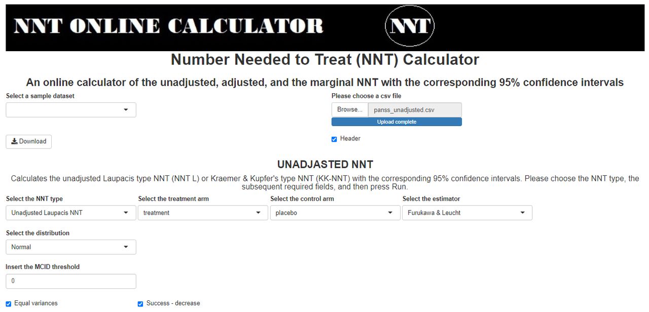
Screenshot of the required fields for the Furukawa and Leucht’s estimator of the unadjusted Laupacis et al’s NNT. The uploaded dataset is the ‘panss_unadjusted.csv’, the selected distribution is normal, the variance equality checkbox is checked, the MCID threshold is set to 0 and the success is defined as a decrease of the outcome variables (the outcome variables are called treatment and placebo, for the treatment and placebo groups, respectively). MCID, minimally clinically important difference; NNT, number needed to treat.
The output consists of the Furukawa and Leucht’s point estimator and the corresponding non-parametric bootstrap-type 95% CI. In this setting, the Furukawa and Leucht’s estimator is appropriate since this dataset was simulated using rounded values of a normal distribution with equal variances. The user may compare this result to the non-parametric and the parametric estimators of the unadjusted NNT in this setting. The estimator can be chosen by changing the estimators to non-parametric and parametric, respectively. The adequacy of the Furukawa and Leucht’s estimator can be assessed by the similarity between this estimator (and its CI) to the non-parametric estimator (with its corresponding CIs). The results of this comparison are presented in online supplemental eTables 1 and 2.
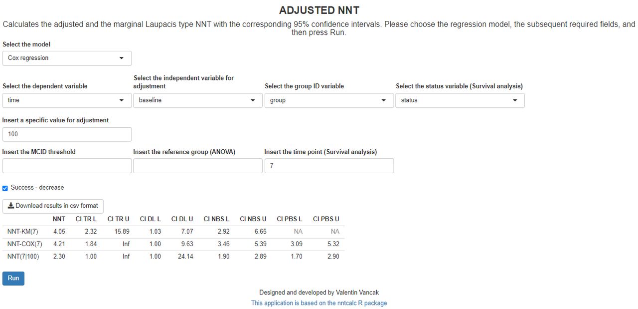
The second scenario corresponds to the Cox model. The required fields for this model are the response variable of the recorded times, and the corresponding status indicator to indicate whether the recorded times are the censoring times (ie, status=0) or the event times (ie, status=1). Other required fieldsare continuous explanatory variable, a fixed timepoint for adjustment, and a specific value for the explanatory variable adjustment. Consider a scenario where the outcome variable is time to an event, for example, time (in months) until discontinuation of treatment, such that the longer the survival time (time to the event), the more efficient the treatment is. Assume two arms: treatment and placebo. Additionally, let the explanatory variable be the PANSS baseline score. Such an adjustment is required since the baseline severity may affect the treatment efficiency (ie, the NNT). In such a setting, we can compute the adjusted NNT for each timepoint and every PANSS baseline score. The simulated dataset ‘panss_survival.csv’ (https://github.com/vancak/nntcalc/tree/main/data) contains the data for this illustration. Without loss of generality, we choose the fixed timepoint to be seven (ie, 7 months after the treatment admission), and the adjusted value of the baseline PANSS Score to be 100 (see figure 2). The results are presented below in table 2.
The output of the Laupacis et al’s NNT estimators for a simulated ‘panss_survival.csv’ dataset

Screenshot of the required fields and the resulted table for estimation of the NNT in survival analysis using the Cox regression model. The adjusted value is the baseline PANSS Score that is set to 100, and the timepoint is set to seven (7 months). Note that for the survival analysis, the calculations may take some time. NNT-KM(7), the Kaplan-Meier-based non-parametric maximum likelihood estimator of the unadjusted NNT for time point 7. NNT-COX(7), Cox regression-based estimator of the marginal NNT for timepoint 7. NNT(7|100), Cox regression-based estimator of the adjusted NNT for timepoint 7 and covariate value of 100. CI DL L, the lower limit of the 95% level delta-method-based CI; CI DL U, the upper limit of the 95% level delta-method-based CI; CI NBS L, lower limit of the 95% level non-parametric-bootstrap-based CI; CI NBS U, the upper limit of the 95% level non-parametric-bootstrap-based CI; CI PBS L, the lower limit of the 95% level parametric-bootstrap-based CI; CI PBS U, the upper limit of the 95% level parametric-bootstrap-based CI; For the unadjusted NNT point estimator, the PBS-based CI limits are not available (NA) since the NNT-KM is a non-parametric estimator. CI TR L, the lower limit of the 95% level transformation-based CI; CI TR U, the upper limit of the 95% level transformation-based CI; MCID, minimally clinically important difference; NNT, number needed to treat; PANSS, Positive and Negative Syndrome Scale. ANOVA, analysis of variance. group ID, group identifier. Inf, Infinity,
The output includes the point estimators of the unadjusted, marginal and the adjusted Laupacis et al’s NNTs, with their corresponding 95% CIs. One can see that the computed adjusted NNT is 2.30. Namely, for patients with a baseline PANSS of 100, we need to treat, on average, 2.30 patients to obtain one more patient who survived 7 months without discontinuing the treatment. The computed marginal NNT is 4.21 and the unadjusted Kaplan-Meier NNT is 4.05. These close results indicate that the Cox model seemed to be appropriate for this data. To compare it to a lower baseline PANSS Score, we set the adjusted value of the baseline PANSS Score to be 80. The fixed time point has remained unchanged at seven. The results are presented below in table 3.
The output of the Laupacis et al’s NNT estimators for a simulated ‘panss_survival.csv’ dataset
One can see that the computed marginal and unadjusted NNTs are the same as in table 2, while the adjusted NNT is 8.75. Namely, for patients with a baseline PANSS of 80, we need to treat, on average, 8.75 patients to obtain one more patient who survived 7 months without discontinuing the treatment. In other words, the higher the baseline PANSS, the more efficient the treatment is. This result is consistent with research showing that higher PANSS severity at baseline corresponds with more change.6
Discussion
We explained the unadjusted, adjusted and marginal NNT and extended our R package with a corresponding web application that provides researchers and clinicians with an easy-to-use user interface to compute the NNT Index for different models in different settings. We aim to show researchers and clinicians how to compute the unadjusted, adjusted and marginal NNT with their corresponding 95% CIs, which provide point-precision bounds in commonly encountered data structures and statistical models. The users can replicate the examples illustrated in this paper by using the application with the simulated datasets that are available online.
Guidelines for using the application can be derived from recent studies. Evidence based on simulation studies, mathematical proofs and NNT research (eg, Vancak et al 5) suggests using the delta-method-based or the bootstrap-based CIs for almost all examined models, except for the marginal NNT in survival analysis. For the marginal NNT in survival analysis, the delta-method-based CIs seemed to perform better than the alternatives; therefore, they are the recommended CI type. Another issue addresses the possible misuse of the application by fitting the wrong model to the data. This problem is also known as the model mis-specification problem and was addressed in recent NNT statistical research.5 A rule of thumb which we can provide is to check whether the point estimators of the marginal and unadjusted NNTs differ significantly. If such a difference occurs, it is likely an indication of model mis-specification, and therefore the use of the non-parametric unadjusted NNT is recommended.
The current version of the application has two main limitations. First, the available models are restricted to five commonly used models. Second, for the survival analysis, the limits of the bootstrap-type CIs for the marginal NNT may differ from the limits of the analytical-type CIs. While the bootstrap-type CIs tend to be more stable, they usually suffer from under coverage. Therefore, despite its imperfection, we recommend using the delta-method-based CIs for the marginal and adjusted NNT in survival analysis rather than the bootstrap-type alternatives.
In conclusion, the current manuscript provides clinicians an understanding, guidelines and an application to compute the NNT in various scenarios.
Ethics statements
Patient consent for publication
References
Supplementary materials
Supplementary Data
This web only file has been produced by the BMJ Publishing Group from an electronic file supplied by the author(s) and has not been edited for content.
Footnotes
Twitter @szlevine
Contributors VV programmed the web application, simulated the datasets and drafted the manuscript. SZL and YG, who are the PhD advisors of VV, edited the manuscript, guided the process and helped conceptualise the study. All authors contributed to and have approved the final manuscript.
Funding The authors have not declared a specific grant for this research from any funding agency in the public, commercial or not-for-profit sectors.
Competing interests None declared.
Provenance and peer review Not commissioned; externally peer reviewed.
Supplemental material This content has been supplied by the author(s). It has not been vetted by BMJ Publishing Group Limited (BMJ) and may not have been peer-reviewed. Any opinions or recommendations discussed are solely those of the author(s) and are not endorsed by BMJ. BMJ disclaims all liability and responsibility arising from any reliance placed on the content. Where the content includes any translated material, BMJ does not warrant the accuracy and reliability of the translations (including but not limited to local regulations, clinical guidelines, terminology, drug names and drug dosages), and is not responsible for any error and/or omissions arising from translation and adaptation or otherwise.