Article Text
Abstract
Objective Meta-analysis is of fundamental importance to obtain an unbiased assessment of the available evidence. In general, the use of meta-analysis has been increasing over the last three decades with mental health as a major research topic. It is then essential to well understand its methodology and interpret its results. In this publication, we describe how to perform a meta-analysis with the freely available statistical software environment R, using a working example taken from the field of mental health.
Methods R package meta is used to conduct standard meta-analysis. Sensitivity analyses for missing binary outcome data and potential selection bias are conducted with R package metasens. All essential R commands are provided and clearly described to conduct and report analyses.
Results The working example considers a binary outcome: we show how to conduct a fixed effect and random effects meta-analysis and subgroup analysis, produce a forest and funnel plot and to test and adjust for funnel plot asymmetry. All these steps work similar for other outcome types.
Conclusions R represents a powerful and flexible tool to conduct meta-analyses. This publication gives a brief glimpse into the topic and provides directions to more advanced meta-analysis methods available in R.
Statistics from Altmetric.com
Introduction
Evidence synthesis is the basis for decision making in a large range of applications including the fields of medicine, psychology and economics.1 Systematic reviews and meta-analysis as statistical method to combine results are cornerstones to yield an unbiased assessment of the available evidence.2 In general, the use of meta-analysis has been increasing over the last three decades with mental health as a major research topic, for example, in Cochrane reviews.3
The freely available statistical software environment R4 (https://www.r-project.org) and the commercial software Stata5 provide the largest collection of statistical methods for meta-analysis. RStudio (https://www.rstudio.com/) is a popular and highly recommended integrated development environment for R providing menu-driven tools for plotting, a history of previous R commands, data management and the installation and update of R packages.
An introduction to meta-analysis with Stata has been published in Evidence-Based Mental Health 6 with specific focus on the challenges in the conduct and interpretation of meta-analysis when outcome data are missing and when small-study effects occur.
In this publication, we replicate these analyses in R using the packages meta7 and metasens.8
In the following, we present R commands to:
Install R packages for meta-analysis.
Conduct a meta-analysis when the outcome of interest is binary.
Assess the impact of missing outcome data.
Assess and account for small-study effects.
Methods
Before conducting a meta-analysis, the R packages meta and metasens need to be installed,9 which include all functions to perform the analyses and to create the figures presented in this publication.
insta l l .packages(c( “ meta ”, “ metasens ” ))
Using this first R command, we would like to mention three general properties of R commands. First, we use brackets in order to execute an R function, here instal l .packages(); the command instal l .packages (without brackets) would show the definition of the function. Second, the argument of an R function can be another R function; here we use the function c() to combine the names of R packages. Third, function arguments are separated by commas that is visible in the call of function c(). RStudio users can also install packages via the menu: Tools ->Install Packages…
The library function can be used to make the R packages available in the current session:
library(meta)
library(metasens)
A brief and very helpful overview of R package meta is provided by the R command help(meta). Among other things, the overview mentions that we can use the settings.meta function to define default settings for the current R session. In this publication, we want to print all results with two significant digits: settings.meta ( digits = 2 ) .
The dataset used in this paper comes from a Cochrane review evaluating the effect of haloperidol in the treatment of symptoms of schizophrenia.10 It has already been used to assess the impact of missing data on clinical outcomes11 and as working example in Chaimani et al.6 It consists of 17 trials comparing haloperidol and placebo, the outcome of interest is clinical improvement and the chosen measure of association is the risk ratio (RR), with an RR larger than 1 meaning that haloperidol is better than placebo.
The information available for each trial, along with the name of the first author (author) and the year of publication (year), is:
The number of participants who responded in the haloperidol arm (resp.h) and in the placebo arm (resp.p).
The number of participants who failed to respond in the haloperidol arm (fail.h) and in the placebo arm (fail.p).
The number of participants who dropped out, for which the outcome is missing, in either arm (drop.h, drop.p).
The dataset contained in ref 10 is available in online supplementary file 1 and can be imported with the following R command, given it is stored in the working directory of the R session: joy = read .csv( “ Joy2006.txt ” ) .
Supplemental material
The function read.csv has several arguments; however, we only specify the name of the text file with the dataset. RStudio users can use the menu to import a dataset: File ->Import Dataset ->From Text (base)… In RStudio, by default, the name of the R dataset is identical to the filename without the extension. Accordingly, the name of the dataset must be set to ‘joy’ in the import wizard in order to run the subsequent R commands.
A new R object joy is created that can be viewed by simply typing: joy .
Alternatively, we can see the data in spreadsheet format: View(joy) .
Or get an overview of the structure of the data (eg, class, dimension, listing and format of variables): str(joy) .
Some studies have participants with missing information due to drop outs (variables drop.h and drop.p). Later, we want to conduct a subgroup analysis of studies with and without missing data and therefore add a new variable with this information to the dataset:
joy$ miss = ifelse ((joy$drop.h + joy$drop.p) == 0 , c( “ Without missing data ” ), c( “ With missing data ” )) .
In general, it is recommended to add all variables that will be used in analyses to the dataset before conducting a meta-analysis. Note, we access single variables in a dataset by using the dollar sign.
A comprehensive description of R features for meta-analysis can be found in Schwarzer et al.9
Fixed effect and random effects meta-analysis
The outcome of interest, that is, clinical improvement, is binary and the brief overview provided by help(meta) reveals that the appropriate R function is metabin.
m.publ = metabin (resp.h, resp.h + fail .h , resp.p, resp.p + fail .p, data = joy, studlab = paste 0 (author, “ ( ”, year, “ )”), method.tau = “ PM ” )
This command creates a new R object, named m.publ, which is a list containing several components describing the meta-analysis that can be accessed with minimum input by the user. By default, the RR is used in metabin as the effect measure, and it is not necessary to specify this explicitly (which could be done setting the argument sm = “ RR ”).
The first four arguments of metabin are mandatory and define the variables containing the number of patients who experienced a clinical improvement and the number of randomised patients (for which we have the information), for the experimental arm and the control arm, respectively. The function performs both fixed effect and random effects meta-analysis,12 using the dataset joy (argument data). The argument studlab defines study labels that are printed in the output and shown in the forest plot, here as the name of the first author and the publication year. The default method to calculate the fixed effect estimate is Mantel-Haenszel.13 The inverse variance weighting could be used for pooling by specifying method = “ Inverse ”, which was used in Chaimani et al.6 The method to estimate the between-study variance in the random effects model can be specified with the argument method.tau; in this example we chose the method by Paule and Mandel,14 which is a recommended method for binary outcomes.15
The result can be viewed by typing m.publ or print(m.publ). The second command could be extended to fine tune the printout by using additional arguments (see help(print.meta)).
We use the following command to generate the forest plot:
forest(m.publ, sortvar = year, prediction = TRUE , label.left = “ Favo u rs placebo ” , label.right = “ Favo u rs haloperidol ” ) .
Only the first argument providing the meta-analysis object m.publ is mandatory. The argument sortvar orders the studies according to the values of the specified variable, in this case by increasing year of publication. The argument prediction = TRUE indicates that a prediction interval16 should be shown in the forest plot. The arguments label.left and label.right specify labels printed at the bottom of the forest plot to simplify its interpretation. A vast number of additional arguments exists to modify the forest plot (see help(forest.meta)).
Assessing the impact of missing outcome data
In order to understand if the results of studies with missing data differed from studies without missing data, a subgroup analysis can be done through the command:
m.publ.sub = update (m.publ, byvar = miss, print.byvar = FALSE ) .
The meta-analysis object m.publ is updated and saved in a new object m.publ.sub. The argument byvar indicates the grouping variable miss, added above to the dataset. The argument print.byvar is used to suppress the printing of the variable name in the subgroup label.
To explore the impact of missing outcome data on the results, several imputation methods have been proposed,11 17 which are available in the function metamiss of the metasens package.
In metamiss, the number of observations with missing outcomes must be provided for the two treatment groups (in our example the variables drop.h and drop.p). The imputation method is specified with argument method.miss, and may be one of the following:
“ GH ” method by Gamble and Hollis.18
“ IMOR ” based on group-specific Informative Missingness Odds Ratios (IMORs).
“ 0 ” imputed as no events, (i.e., 0) – default method (Imputed Case Analysis (ICA)-0).
“ 1 ” imputed as events (ie, 1) (ICA-1).
“ pc ” based on observed risk in control group (ICA-pc).
“ pe ” based on observed risk in experimental group (ICA-pe).
“ p ” based on group-specific risks (ICA-p).
“ b ” best case scenario for experimental group (ICA-b).
“ w ” worst case scenario for experimental group (ICA-w).
For example, the following command will impute missing data as events: mmiss.1 = metamiss (m.publ, drop.h, drop.p, method.miss = “ 1 ” ) .
The method by Gamble and Hollis18 is based on uncertainty intervals for individual studies, assuming best and worst case scenarios for the missing data. Inflated SEs are calculated from the uncertainty intervals and then considered in a generic inverse variance meta-analysis instead of the SEs from the available case meta-analysis.
All other methods are based on the Informative Missingness Odds Ratios (IMOR), defined as the odds of an event in the missing group over the odds of an event in the observed group11 (eg, an IMOR of 2 means that the odds for an event is assumed to be twice as likely for missing observations).
For method.miss = “ IMOR ”, the IMORs in the experimental (argument IMOR.e) and control group (argument IMOR.c) must be specified; if both values are assumed to be equal, only argument IMOR.e has to be provided. For all other methods, the input for arguments IMOR.e and IMOR.c is ignored as these values are determined by the respective imputation method (see table 2 in ref 11). It must be specified whether the outcome is beneficial (argument small.values = “ good ”) or harmful (small.values = “ bad ”) when best or worst case scenarios are chosen, that is, if argument method.miss is equal to “ b ” or “ w ”.
Assessing and accounting for small-study effects
Sometimes small studies show different, often larger, treatment effects compared with the large ones. The association between size and effect in meta-analysis is referred to as small-study effects.19
The first step to assess the presence of small-study effects is usually to have a look at the funnel plot, where effect estimates are plotted against a measure of precision, usually the SE of the effect estimate. This can be done through the function funnel.meta with the meta-analysis object as input: funnel(m.publ) .
An asymmetric funnel plot indicates that small-study effects are present. Publication bias, though the most popular, is only one of several possible reasons for asymmetry.20 A contour-enhanced funnel plot may help to distinguish if asymmetry is due to publication bias, by adding lines representing regions where a test of treatment effect is significant.21 In order to generate such a contour-enhanced funnel plot, the argument contour.levels must be specified: funnel (m.publ, contour.levels = c (0.9, 0.95, 0.99), col.contour = c ( “ darkgray ”, “ gr a y ”, “ lightgray ” )) .
Several tests, often referred to as tests for small-study effects or tests for funnel plot asymmetry, have been proposed to assess whether the association between estimated effects and study size is larger than might be expected by chance.20 22 These tests typically have low power, meaning that even when they do not support the presence of asymmetry, bias cannot be excluded. Accordingly, they should be used only if the number of included studies is 10 or larger.20 The Harbord score test, where the test statistic is based on a weighted linear regression of the efficient score on its SE,23 is applied in this example: metabias (m.publ, method.bias = “ score ” ) .
As usual, the first argument is the object created through metabin, while the argument method.bias specifies the test to be used: “ score ” is for the Harbord test. The metabias function provides several other methods for testing funnel plot asymmetry (see help(metabias)).
Once the presence of asymmetry in the funnel plot has been detected, it is also possible to conduct sensitivity analyses to adjust the effect estimate for this bias. Different methods exist22; in this paper, we report the more established trim-and-fill method24 and the method of adjusting by regression.25 Another more advanced method is the Copas selection model,26 which we do not treat here.
The trim-and-fill method, 1) removes/“trims” studies from the funnel plot until it becomes symmetric 2) adds/“fills” mirror images of removed studies (ie, unpublished studies) to the original funnel plot and 3) calculates the adjusted effect estimate based on original and added studies. The function to apply is trimfill: tf.publ = trimfill (m.publ) .
With this command, a new object is created, named tf.publ. The results can be shown by typing tf.publ or summary (tf.publ) to get a brief summary, and a corresponding funnel plot can be created: funnel (tf.publ) .
A specific implementation of the “adjusting by regression” method, called “limit meta-analysis”, is described in detail in ref 25. The underlying model, motivated by Egger’s test,20 is an extended random effects model with an additional parameter alpha representing possible small study effects (funnel plot asymmetry) by allowing the treatment effect to depend on the SE. More explicitly, alpha is the expected shift in the standardised treatment effect if precision is very small. The model provides an adjusted treatment effect estimate that is interpreted as the limit treatment effect for a study with infinite precision. Graphically, this means adding to the funnel plot a curve from the bottom to a point at the top which marks the adjusted treatment effect estimate. The corresponding function is limitmeta: l1.publ = limitmeta(m.publ) .
A new object, named l1.publ, is created. As usual, the results can be viewed by typing its name. The funnel plot can be created using the command: funnel(l1.publ) .
Results
R commands for meta-analysis and sensitivity analyses have been described in the previous section. In order to produce the figures in this publication, we slightly modified some of the R commands introduced before and had to run some additional computations. All R commands used to perform the analyses in this section—including R code for the figures—can be found in the online supplementary file 2.
Supplemental material
Fixed effect and random effects meta-analysis
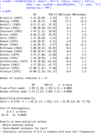
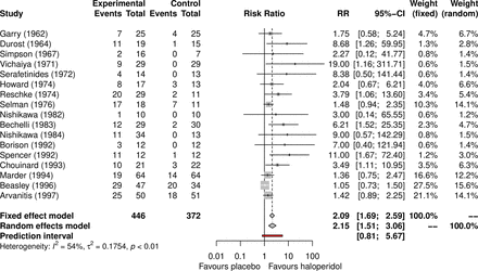
The metabin function printout is displayed in figure 1 containing all basic meta-analysis information (individual study results, fixed effect and random effects results, heterogeneity information and details on meta-analytical method). The forest plot showing the results of both fixed effect and random effects meta-analysis considering the available cases is given in figure 2. For both models, the diamonds presenting the estimated RRs and confidence limits do not cross the line of no effect, suggesting that haloperidol is significantly more effective than placebo. However, this result should be taken with caution: the prediction interval, incorporating the between-study heterogeneity, crosses the line of no effect, revealing that placebo might be superior to haloperidol in a future study.
Printout of metabin function.
Forest plot showing the results of fixed effect and random effects meta-analysis (available case analysis).
Some CIs in the forest plot do not overlap, and the test of heterogeneity (p=0.004) also suggests the presence of heterogeneous results. The heterogeneity statistic I2 is 54%, indicative of moderate heterogeneity; its CI ranges from 21% to 74%, denoting potentially unimportant to substantial heterogeneity (ref 13, section 9.5.2).13 As expected, the CI for the summary estimate from the random effects model is wider compared with the one from the fixed effect model, but the two results differ only slightly in terms of magnitude.
Assessing the impact of missing outcome data
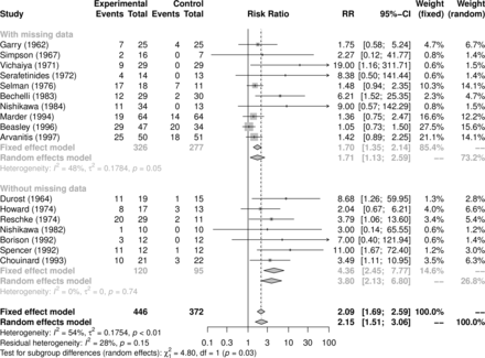
The forest plot for the subgroup analysis by presence of missing data in the studies is shown in figure 3. Though both subgroups give significant results, studies without missing data report a larger haloperidol effect compared with the studies with missing data. Not all CIs for the subgroup estimates include the respective overall effect (in a negligible way for the random effects model), and the test for subgroup differences under the random effects model displayed in the forest plot support the visual detection, suggesting that missing data might have some impact on the results (p=0.03). A reason may be that patients randomised to placebo are more likely to withdraw from the study because of lack of efficacy compared with the patients randomised to an active treatment. If these patients were lost to follow-up, their poor responses were not seen, and the treatment effects in these studies were underestimated. For example, two studies (Beasley and Selman) with a larger number of missing observations in the placebo group have rather small treatment estimates.
Forest plot showing the subgroup analysis by presence of missing data (available case analysis).
In order to better understand how missing data might have influenced the results, more appropriate methods are provided by metamiss making different assumptions on the missingness mechanism. The results for the random effects model are presented in figure 4. Overall, results are rather similar with RRs ranging from 1.90 to 2.64 for the extreme worst and best case scenarios. All sensitivity analyses still suggest that haloperidol is better than placebo in improving the symptoms of schizophrenia, indicating that missing outcome data are not a serious problem in this dataset.
Summary risk ratios according to different assumptions about mechanism of missingness.
Assessing and accounting for small-study effects
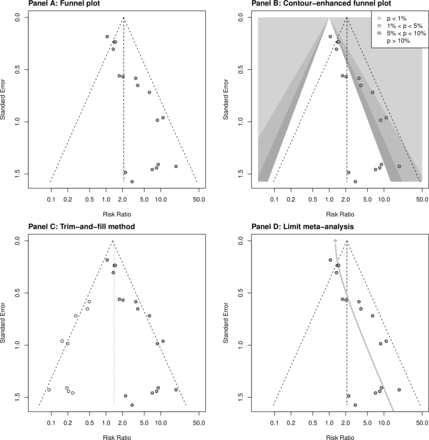
The funnel plot is shown in figure 5 (panel A). The fixed effect model is represented by a dashed line on which the funnel is centred, while the random effects model estimate is indicated by a dotted line. As in our example, both estimates are similar; they cannot be well distinguished. The funnel plot clearly looks asymmetric; however, based on the contour-enhanced funnel plot (figure 5, panel B), publication bias seems not to be the dominant factor for the asymmetry as most small studies with large SEs lie in the white area corresponding to non-significant treatment estimates. The Harbord test is highly significant (p<0.001), supporting the presence of small-study effects.
Funnel plot and various methods to evaluate funnel plot asymmetry.
The trim-and-fill method added nine studies to the meta-analysis (figure 5, panel C), leading to an adjusted random effects estimate RR=1.40 (0.83–2.38) suggesting a non-significant benefit of haloperidol compared with placebo.
The result of the limit meta-analysis is shown in figure 5, panel D. The grey curve indicates some funnel plot asymmetry: it begins (at the bottom) with a considerable deviation from the random effects estimate caused by the small studies and balances this by approaching a point (at the top) left to the random effects estimate, representing the adjusted estimate RR=1.29 (0.93–1.79), again covering the line of no effect.
Discussion
Meta-analysis is a fundamental tool for evidence-based medicine, making it essential to well understand its methodology and interpret its results. Nowadays several software options are available to perform a meta-analysis. In this paper, we aimed to give a brief introduction on how to conduct a meta-analysis in the freely available software R using the meta and metasens packages, which provide a user-friendly implementation of meta-analysis methods. The meta package has been developed by the last author to communicate meta-analysis results to clinical colleagues in the context of Cochrane reviews.
For illustration, we used an example with a binary outcome and showed how to conduct a meta-analysis and subgroup analysis, produce a forest and funnel plot and to test and adjust for funnel plot asymmetry. All these steps work similar for other outcome types, for example, R function metacont can be used for continuous outcomes. Additionally, we conducted a sensitivity analysis for missing binary outcomes using R function metamiss.
In our example, all sensitivity analyses for missing data resulted in similar results supporting the benefit of haloperidol over placebo despite very different assumptions on the missingness mechanism. However, the evaluation of funnel plot asymmetry revealed a small-study effect that—according to the contour-enhanced funnel plot—cannot be attributed to publication bias. While all sensitivity analyses adjusting for selection bias resulted in non-significant treatment estimates, we would not like to interpret these results too much as clinical heterogeneity could be another explanation for the small-study effect.22 A deeper knowledge of the condition under study, of the treatment and the settings in which it was administered in different trials could help to identify the probable reason for asymmetry in the funnel plot.
In this publication, we could only provide a brief glimpse into statistical methods for meta-analysis available in R. The interested reader can see this publication as a starting point for other (more advanced) meta-analysis methods available in R. An overview of R packages for meta-analysis is provided on the website https://cran.r-project.org/view=MetaAnalysis. We would like to only briefly mention two R packages from this list. R package metafor27 is another general package for meta-analysis, which in addition provides methods for multilevel meta-analysis28 as well as multivariate meta-analysis.29 R package netmeta30 implements a frequentist method for network meta-analysis and is as of today the most comprehensive R package for network meta-analysis.
References
Footnotes
Contributors SB drafted the manuscript and performed analyses; GR and GS critically revised the manuscript and reviewed the analyses.
Funding The authors have not declared a specific grant for this research from any funding agency in the public, commercial or not-for-profit sectors.
Competing interests None declared.
Patient consent for publication Not required.
Provenance and peer review Not commissioned; externally peer reviewed.


